


*** INCOMPLETE ***
There are three major kinds of power supplies: unregulated (also called brute force), linear regulated, and switching. A fourth type of power supply circuit called the ripple-regulated, is a hybrid between the "brute force" and "switching" designs, and merits a subsection to itself.
An unregulated power supply is the most rudimentary type, consisting of a transformer, rectifier, and low-pass filter. These power supplies typically exhibit a lot of ripple voltage (i.e. rapidly-varying instability) and other AC "noise" superimposed on the DC power. If the input voltage varies, the output voltage will vary by a proportional amount. The advantage of an unregulated supply is that it's cheap, simple, and efficient.
A linear regulated supply is simply a "brute force" (unregulated) power supply followed by a transistor circuit operating in its "active," or "linear" mode, hence the name linear regulator. (Obvious in retrospect, isn't it?) A typical linear regulator is designed to output a fixed voltage for a wide range of input voltages, and it simply drops any excess input voltage to allow a maximum output voltage to the load. This excess voltage drop results in significant power dissipation in the form of heat. If the input voltage gets too low, the transistor circuit will lose regulation, meaning that it will fail to keep the voltage steady. It can only drop excess voltage, not make up for a deficiency in voltage from the brute force section of the circuit. Therefore, you have to keep the input voltage at least 1 to 3 volts higher than the desired output, depending on the regulator type. This means the power equivalent of at least 1 to 3 volts multiplied by the full load current will be dissipated by the regulator circuit, generating a lot of heat. This makes linear regulated power supplies rather inefficient. Also, to get rid of all that heat they have to use large heat sinks which makes them large, heavy, and expensive.
A switching regulated power supply ("switcher") is an effort to realize the advantages of both brute force and linear regulated designs (small, efficient, and cheap, but also "clean," stable output voltage). Switching power supplies work on the principle of rectifying the incoming AC power line voltage into DC, re-converting it into high-frequency square-wave AC through transistors operated as on/off switches, stepping that AC voltage up or down by using a lightweight transformer, then rectifying the transformer's AC output into DC and filtering for final output. Voltage regulation is achieved by altering the "duty cycle" of the DC-to-AC inversion on the transformer's primary side. In addition to lighter weight because of a smaller transformer core, switchers have another tremendous advantage over the prior two designs: this type of power supply can be made so totally independent of the input voltage that it can work on any electric power system in the world; these are called "universal" power supplies.
The downside of switchers is that they are more complex, and due to their operation they tend to generate a lot of high-frequency AC "noise" on the power line. Most switchers also have significant ripple voltage on their outputs. With the cheaper types, this noise and ripple can be as bad as for an unregulated power supply; such low-end switchers aren't worthless, because they still provide a stable average output voltage, and there's the "universal" input capability.
Expensive switchers are ripple-free and have noise nearly as low as for some a linear types; these switchers tend to be as expensive as linear supplies. The reason to use an expensive switcher instead of a good linear is if you need universal power system compatibility or high efficiency. High efficiency, light weight, and small size are the reasons switching power supplies are almost univerally used for powering digital computer circuitry.
A ripple-regulated power supply is an alternative to the linear regulated design scheme: a "brute force" power supply (transformer, rectifier, filter) constitutes the "front end" of the circuit, but a transistor operated strictly in its on/off (saturation/cutoff) modes transfers DC power to a large capacitor as needed to maintain the output voltage between a high and a low setpoint. As in switchers, the transistor in a ripple regulator never passes current while in its "active," or "linear," mode for any substantial length of time, meaning that very little energy will be wasted in the form of heat. However, the biggest drawback to this regulation scheme is the necessary presence of some ripple voltage on the output, as the DC voltage varies between the two voltage control setpoints. Also, this ripple voltage varies in frequency depending on load current, which makes final filtering of the DC power more difficult.
Ripple regulator circuits tend to be quite a bit simpler than switcher circuitry, and they need not handle the high power line voltages that switcher transistors must handle, making them safer to work on.
When someone mentions the word "computer," a digital device is what usually comes to mind. Digital circuits represent numerical quantities in binary format: patterns of 1's and 0's represented by a multitude of transistor circuits operating in saturated or cutoff states. However, analog circuitry may also be used to represent numerical quantities and perform mathematical calculations, by using variable voltage signals instead of discrete on/off states.
Here is a simple example of binary (digital) representation versus analog representation of the number "twenty-five:"
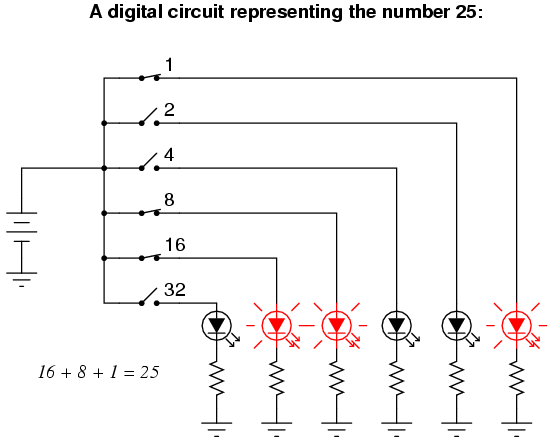
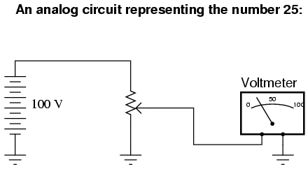
Digital circuits are very different from circuits built on analog principles. Digital computational circuits can be incredibly complex, and calculations must often be performed in sequential "steps" to obtain a final answer, much as a human being would perform arithmetical calculations in steps with pencil and paper. Analog computational circuits, on the other hand, are quite simple in comparison, and perform their calculations in continuous, real-time fashion. There is a disadvantage to using analog circuitry to represent numbers, though: imprecision. The digital circuit shown above is representing the number twenty-five, precisely. The analog circuit shown above may or may not be exactly calibrated to 25.000 volts, but is subject to "drift" and error.
In applications where precision is not critical, analog computational circuits are very practical and elegant. Shown here are a few op-amp circuits for performing analog computation:
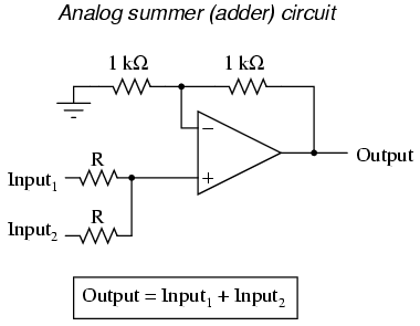
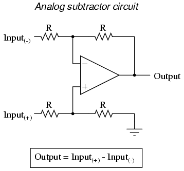
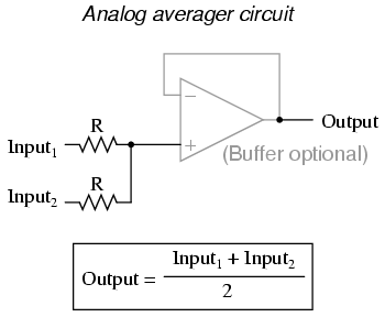
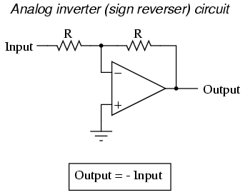
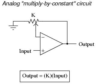
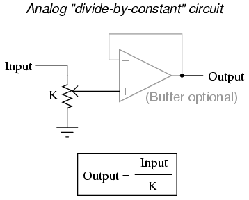
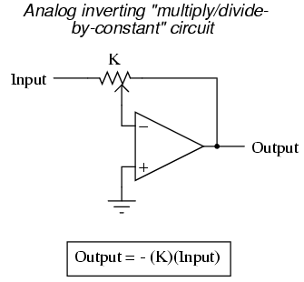
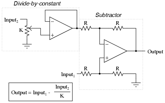
Each of these circuits may be used in modular fashion to create a circuit capable of multiple calculations. For instance, suppose that we needed to subtract a certain fraction of one variable from another variable. By combining a divide-by-constant circuit with a subtractor circuit, we could obtain the required function:
Devices called analog computers used to be common in universities and engineering shops, where dozens of op-amp circuits could be "patched" together with removable jumper wires to model mathematical statements, usually for the purpose of simulating some physical process whose underlying equations were known. Digital computers have made analog computers all but obsolete, but analog computational circuitry cannot be beaten by digital in terms of sheer elegance and economy of necessary components.
Analog computational circuitry excels at performing the calculus operations integration and differentiation with respect to time, by using capacitors in an op-amp feedback loop. To fully understand these circuits' operation and applications, though, we must first grasp the meaning of these fundamental calculus concepts. Fortunately, the application of op-amp circuits to real-world problems involving calculus serves as an excellent means to teach basic calculus. In the words of John I. Smith, taken from his outstanding textbook, Modern Operational Circuit Design:
"A note of encouragement is offered to certain readers: integral calculus is one of the mathematical disciplines that operational [amplifier] circuitry exploits and, in the process, rather demolishes as a barrier to understanding." (pg. 4)
Mr. Smith's sentiments on the pedagogical value of analog circuitry as a learning tool for mathematics are not unique. Consider the opinion of engineer George Fox Lang, in an article he wrote for the August 2000 issue of the journal Sound and Vibration, entitled, "Analog was not a Computer Trademark!":
"Creating a real physical entity (a circuit) governed by a particular set of equations and interacting with it provides unique insight into those mathematical statements. There is no better way to develop a "gut feel" for the interplay between physics and mathematics than to experience such an interaction. The analog computer was a powerful interdisciplinary teaching tool; its obsolescence is mourned by many educators in a variety of fields." (pg. 23)
Differentiation is the first operation typically learned by beginning calculus students. Simply put, differentiation is determining the rate-of-change of one variable as it relates to another. In analog differentiator circuits, the independent variable is time, and so the rates of change we're dealing with are rates of change of some measured quantity over time.
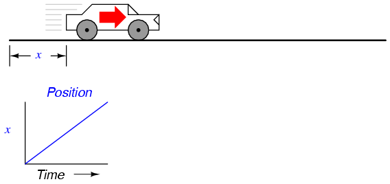
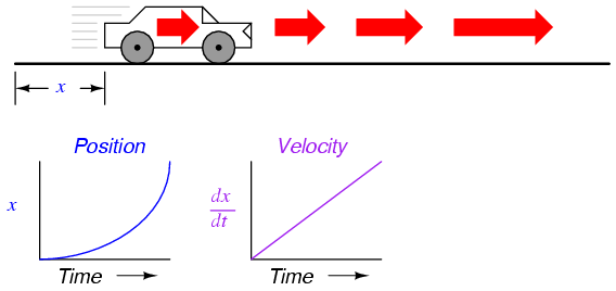
Suppose we were to measure the position of a car, traveling in a direct path (no turns), from its starting point. Let us call this measurement, x. If the car moves at a rate such that its distance from "start" increases steadily over time, its position will plot on a graph as a linear function (straight line):
If we were to calculate the derivative of the car's position with respect to time (that is, determine the rate-of-change of the car's position over time), we would arrive at a quantity representing the car's velocity. The differentiation function is represented by the fractional notation d/d, so when differentiating position (x) with respect to time (t), we denote the result (the derivative) as dx/dt:
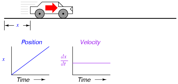
For a linear graph of x over time, the derivate of position (dx/dt), otherwise and more commonly known as velocity, will be a flat line, unchanging in value. The derivative of a mathematical function may be graphically understood as its slope when plotted on a graph, and here we can see that the position (x) graph has a constant slope, which means that its derivative (dx/dt) must be constant over time.
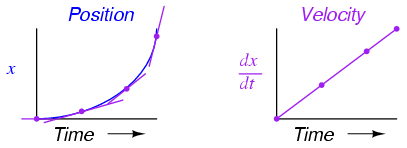
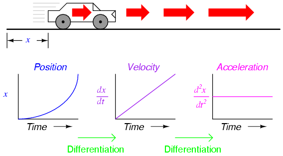
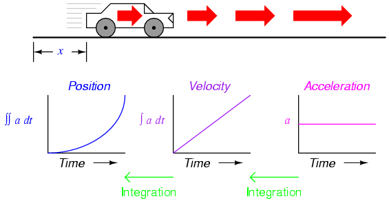
Now, suppose the distance traveled by the car increased exponentially over time: that is, it began its travel in slow movements, but covered more additional distance with each passing period in time. We would then see that the derivative of position (dx/dt), or velocity, would not be constant over time, but would increase:
The height of points on the velocity graph correspond to the rates-of-change, or slope, of points at corresponding times on the position graph:
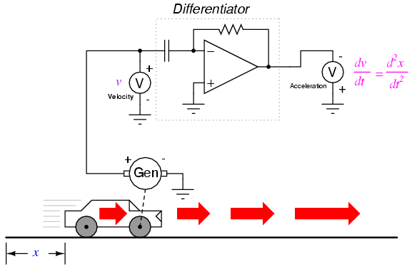
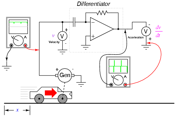
What does this have to do with analog electronic circuits? Well, if we were to have an analog voltage signal represent the car's position (think of a huge potentiometer whose wiper was attached to the car, generating a voltage proportional to the car's position), we could connect a differentiator circuit to this signal and have the circuit continuously calculate the car's velocity, displaying the result via a voltmeter connected to the differentiator circuit's output:
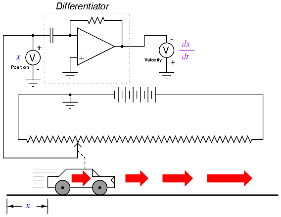
Recall from the last chapter that a differentiator circuit outputs a voltage proportional to the input voltage's rate-of-change over time. Thus, if the input voltage is changing over time at a constant rate, the output voltage will be at a constant value. If the car moves in such a way that its elapsed distance over time builds up at a steady rate, then that means the car is traveling at a constant velocity, and the differentiator circuit will output a constant voltage proportional to that velocity. If the car's elapsed distance over time changes in a non-steady manner, the differentiator circuit's output will likewise be non-steady, but always at a level representative of the input's rate-of-change over time.
Note that the voltmeter registering velocity (at the output of the differentiator circuit) is connected in "reverse" polarity to the output of the op-amp. This is because the differentiator circuit shown is inverting: outputting a negative voltage for a positive input voltage rate-of-change. If we wish to have the voltmeter register a positive value for velocity, it will have to be connected to the op-amp as shown. As impractical as it may be to connect a giant potentiometer to a moving object such as an automobile, the concept should be clear: by electronically performing the calculus function of differentiation on a signal representing position, we obtain a signal representing velocity.
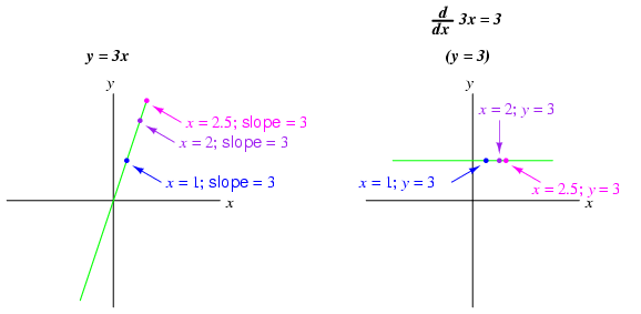
Beginning calculus students learn symbolic techniques for differentiation. However, this requires that the equation describing the original graph be known. For example, calculus students learn how to take a function such as y = 3x and find its derivative, 3, simply by manipulating the equation. We may verify the accuracy of this manipulation by comparing the graphs of the two functions:
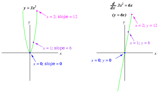
Nonlinear functions such as y = 3x2 may also be differentiated by symbolic means. In this case, the derivative of y = 3x2 is 6x:
In real life, though, we often cannot describe the behavior of any physical event by a simple equation like y = 3x, and so symbolic differentiation of the type learned by calculus students may be impossible to apply to a physical measurement. If someone wished to determine the derivative of our hypothetical car's position (dx/dt = velocity) by symbolic means, they would first have to obtain an equation describing the car's position over time, based on position measurements taken from a real experiment -- a nearly impossible task unless the car is operated under carefully controlled conditions leading to a very simple position graph. However, an analog differentiator circuit, by exploiting the behavior of a capacitor with respect to voltage, current, and time i = C(dv/dt), naturally differentiates any real signal in relation to time, and would be able to output a signal corresponding to instantaneous velocity (dx/dt) at any moment. By logging the car's position signal along with the differentiator's output signal using a chart recorder or other data acquisition device, both graphs would naturally present themselves for inspection and analysis.
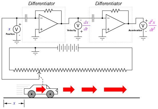
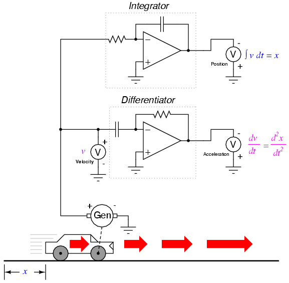
We may take the principle of differentiation one step further by applying it to the velocity signal using another differentiator circuit. In other words, use it to calculate the rate-of-change of velocity, which we know is the rate-of-change of position. What practical measure would we arrive at if we did this? Think of this in terms of the units we use to measure position and velocity. If we were to measure the car's position from its starting point in miles, then we would probably express its velocity in units of miles per hour (dx/dt). If we were to differentiate the velocity (measured in miles per hour), we would end up with a unit of miles per hour per hour. Elementary physics classes teach students about the behavior of falling objects, measuring position in meters, velocity in meters per second, and change in velocity over time in meters per second, per second. This final measure is called acceleration: the rate of change of velocity over time:
The expression d2x/dt2 is called the second derivative of position (x) with regard to time (t). If we were to connect a second differentiator circuit to the output of the first, the last voltmeter would register acceleration:
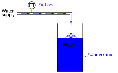
Deriving velocity from position, and acceleration from velocity, we see the principle of differentiation very clearly illustrated. These are not the only physical measurements related to each other in this way, but they are, perhaps, the most common. Another example of calculus in action is the relationship between liquid volume and liquid flow:
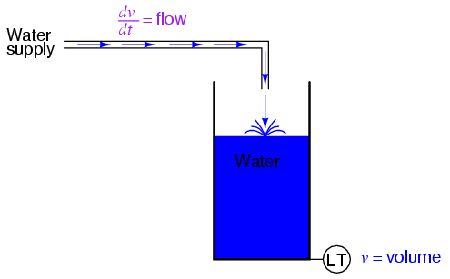
A "Level Transmitter" device mounted on a water storage tank provides a signal directly proportional to water level in the tank, which -- if the tank is of constant cross-sectional area throughout its height -- directly equates water volume stored. If we were to take this volume signal and differentiate it with respect to time (dv/dt), we would obtain a signal proportional to the water flow rate through the pipe carrying water to the tank. A differentiator circuit connected in such a way as to receive this volume signal would produce an output signal proportional to flow, possibly substituting for a flow-measurement device ("Flow Transmitter") installed in the pipe.
Returning to the car experiment, suppose that our hypothetical car were equipped with a tachogenerator on one of the wheels, producing a voltage signal directly proportional to velocity. We could differentiate the signal to obtain acceleration with one circuit, like this:
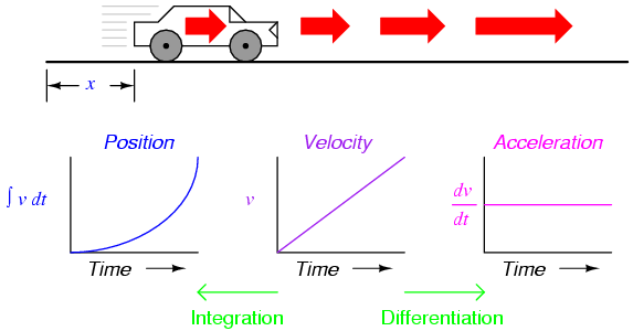
In a sense, the tachogenerator by its very nature differentiates the car's position, generating a voltage proportional to how rapidly the wheel's angular position changes over time. This provides us with a raw signal already representative of velocity, with only a single step of differentiation needed to obtain an acceleration signal. A tachogenerator measuring velocity, of course, is a far more practical example of automobile instrumentation than a giant potentiometer measuring its physical position, but what we gain in practicality we lose in position measurement. No matter how many times we differentiate, we can never infer the car's position from a velocity signal. If the process of differentiation brought us from position to velocity to acceleration, then somehow we need to perform the "reverse" process of differentiation to go from velocity to position. Such a mathematical process does exist, and it is called integration. The "integrator" circuit may be used to perform this function:
Recall from the last chapter that an integrator circuit outputs a voltage whose rate-of-change over time is proportional to the input voltage's magnitude. Thus, given a constant input voltage, the output voltage will change at a constant rate. If the car travels at a constant velocity (constant voltage input to the integrator circuit from the tachogenerator), then its distance traveled will increase steadily as time progresses, and the integrator will output a steadily changing voltage proportional to that distance. If the car's velocity is not constant, then neither will the rate-of-change over time be of the integrator circuit's output, but the output voltage will faithfully represent the amount of distance traveled by the car at any given point in time.
The symbol for integration looks something like a very narrow, cursive letter "S". The equation utilizing this symbol tells us that we are integrating velocity (v) with respect to time (dt), and obtaining position (x) as a result of it.
So, we may express three measures of the car's motion (position, velocity, and acceleration) in terms of velocity (v) just as easily as we could in terms of position (x):
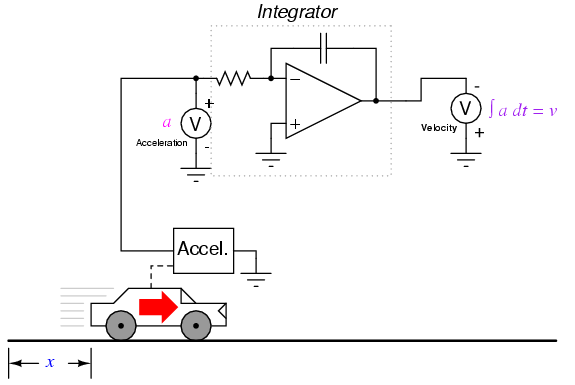
If we had an accelerometer attached to the car, generating a signal proportional to the rate of acceleration or deceleration, we could (hypothetically) obtain a velocity signal with one step of integration, and a position signal with a second step of integration:
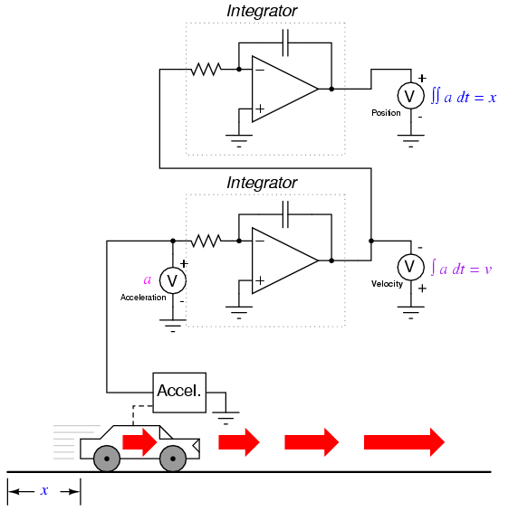
Thus, all three measures of the car's motion (position, velocity, and acceleration) may be expressed in terms of acceleration:
As you might have suspected, the process of integration may be illustrated in, and applied to, other physical systems as well. Take for example the water storage tank and flow example shown earlier. If flow rate is the derivative of tank volume with respect to time (f = dv/dt), then we could also say that volume is the integral of flow rate:
If we were to use a "Flow Transmitter" device to measure water flow, then by integration we could calculate the volume of water accumulated in the tank over time. Although it is theoretically possible to use a capacitive op-amp integrator circuit to derive a volume signal from a flow signal, mechanical and digital electronic "integrator" devices are more practical for reasons of error and drift, and find frequent use in the water treatment and distribution industries.
Just as there are symbolic techniques for differentiation, there are also symbolic techniques for integration, although they tend to be more complex and varied. Applying symbolic integration to a real-world problem like the acceleration of a car, though, is still contingent on the availability of an equation precisely describing the measured signal -- often a difficult or impossible thing to derive from measured data. However, electronic integrator circuits perform this mathematical function continuously, in real time, and for any input signal profile, providing a powerful tool for scientists and engineers.
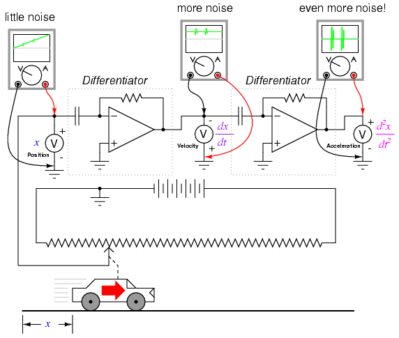
Having said this, there are caveats to the using calculus techniques to derive one type of measurement from another. Differentiation has the undesirable tendency of amplifying "noise" found in the measured variable, since the noise will typically appear as frequencies much higher than the measured variable, and high frequencies by their very nature possess high rates-of-change over time.
To illustrate this problem, suppose we were deriving a measurement of car acceleration from the velocity signal obtained from a tachogenerator with worn brushes or commutator bars. Points of poor contact between brush and commutator will produce momentary "dips" in the tachogenerator's output voltage, and the differentiator circuit connected to it will interpret these dips as very rapid changes in velocity. For a car moving at constant speed -- neither accelerating nor decelerating -- the acceleration signal should be 0 volts, but "noise" in the velocity signal caused by a faulty tachogenerator will cause the differentiated (acceleration) signal to contain "spikes," falsely indicating brief periods of high acceleration and deceleration:
Noise voltage present in a signal to be differentiated need not be of significant amplitude to cause trouble: all that is required is that the noise profile have fast rise or fall times. In other words, any electrical noise with a high dv/dt component will be problematic when differentiated, even if it is of low amplitude.
It should be noted that this problem is not an artifact (an idiosyncratic error of the measuring/computing instrument) of the analog circuitry; rather, it is inherent to the process of differentiation. No matter how we might perform the differentiation, "noise" in the velocity signal will invariably corrupt the output signal. Of course, if we were differentiating a signal twice, as we did to obtain both velocity and acceleration from a position signal, the amplified noise signal output by the first differentiator circuit will be amplified again by the next differentiator, thus compounding the problem:
Integration, on the other hand, does not suffer from this problem, because high-frequency noise tends to be filtered out. One might suppose, then, that we could avoid all trouble by measuring acceleration directly and integrating that signal to obtain velocity; in effect, calculating in "reverse" from the way shown previously:
Unfortunately, following this methodology might lead us into other difficulties, the greatest being a common artifact of analog integrator circuits known as drift. All op-amps have some amount of input bias current, and this current will tend to cause a charge to accumulate on the capacitor in addition to whatever charge accumulates as a result of the input voltage signal. In other words, all analog integrator circuits suffer from the tendency of having their output voltage "drift" or "creep" even when there is absolutely no voltage input, accumulating error over time as a result. Also, imperfect capacitors will tend to lose their stored charge over time due to internal resistance, resulting in "drift" toward zero output voltage. These problems are artifacts of the analog circuitry, and may be eliminated through the use of digital computation.
Circuit artifacts notwithstanding, possible errors may result from the integration of one measurement (such as acceleration) to obtain another (such as velocity) simply because of the way integration works. If the "zero" calibration point of the raw signal sensor is not perfect, it will output a slight positive or negative signal even in conditions when it should output nothing. Consider a car with an imperfectly calibrated accelerometer, or one that is influenced by gravity to detect a slight acceleration unrelated to car motion. Even with a perfect integrating computer, this sensor error will cause the integrator to accumulate error, resulting in an output signal indicating a change of velocity when the car is neither accelerating nor decelerating.
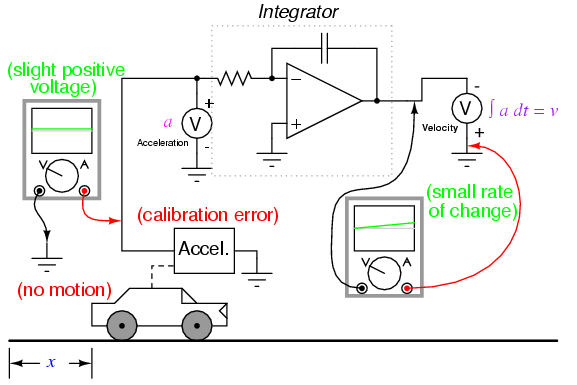
As with differentiation, this error will also compound itself if the integrated signal is passed on to another integrator circuit, since the "drifting" output of the first integrator will very soon present a significant positive or negative signal for the next integrator to integrate. Therefore, care should be taken when integrating sensor signals: if the "zero" adjustment of the sensor is not perfect, the integrated result will drift, even if the integrator circuit itself is perfect. Again, it should be clearly understood that integrator errors such as these are fundamentally errors with the integrator and/or sensor devices themselves, and not inherent to the principle of signal integration. By contrast, differentiator errors (amplification of high-frequency noise) are inherent to the process of differentiation and are impossible to eliminate without completely eliminating input signal noise.
Contributors to this chapter are listed in chronological order of their contributions, from most recent to first. See Appendix 2 (Contributor List) for dates and contact information.
Warren Young (August 2002): Initial idea and text for "Power supply circuits" section. Paragraphs modified by Tony Kuphaldt (changes in vocabulary, plus inclusion of additional concepts).
Lessons In Electric Circuits copyright (C) 2000-2003 Tony R. Kuphaldt, under the terms and conditions of the Design Science License.